
There is an introduction to the nature of the “Hubble tension” in the first part of this article, which covers measurements based on the distance ladder (see https://physbang.com/2026/07/28/hubble-tension-part-1-the-distance-ladder/).
This article looks at how the Cosmic Microwave Background (CMB) can be used to calculate the expansion of the Universe – and therefore the Hubble constant. But first it is useful to cover a bit of the relevant background.
In 1964, two radio engineers working at Bell Labs, Arno Penzias and Robert Wilson, discovered a microwave radio signal that could not be isolated: it seemed to come from every direction. At the same time, theoretical physicists, headed by Robert Dicke at Princeton University, calculated that if the Universe started with a Big Bang (an assumption that was by no means certain at the time) then there ought to be a left-over signal from that event. The signal was predicted to be in the microwave radio region of the electromagnetic spectrum.
The Princeton theory, together with the practical measurements obtained by Penzias and Wilson, came together in the July 1965 issue of Astrophysical Journal Letters when two complementary papers were published on consecutive pages. Together, they cemented the idea that the Universe was created in an event that we now call the Big Bang. Penzias and Wilson subsequently shared the 1978 Nobel Prize for Physics; Dicke was nominated seven times but never won.
Over the decades since then, increasingly detailed maps of the CMB have been created, revealing it to be not-quite uniform. The slight power (temperature) fluctuations seen in the CMB signal, illustrated below, are explained by small density variations in the early Universe.

The density variations implicated in the CMB are in turn explained using the different behaviours of dark matter and baryonic (normal) matter in the early Universe.
Dark matter will clump together under gravitational attraction but baryonic matter contains charged particles that both attract (protons and electrons) and repel (protons and protons, or electrons and electrons) via the exchange of virtual photons. The interplay between these different forces causes the baryonic matter to occupy an expanding volume rather than being attracted to the dark matter.
The temperature at this time was so high that protons and electrons could not combine: they existed as plasma, which also trapped the photons. Not only could the photons not escape but also they couldn’t even move at their usual speed owing to their interactions with the charged particles. All three types of particles had the same velocity, which was the speed of “sound” (particle-to-particle energy transfer) in the plasma. This was the speed at which the baryon-photon wavefront travelled outwards – until the moment when the baryons were able to combine and the region became transparent to photons.
The animation below illustrates this – and is explained below.
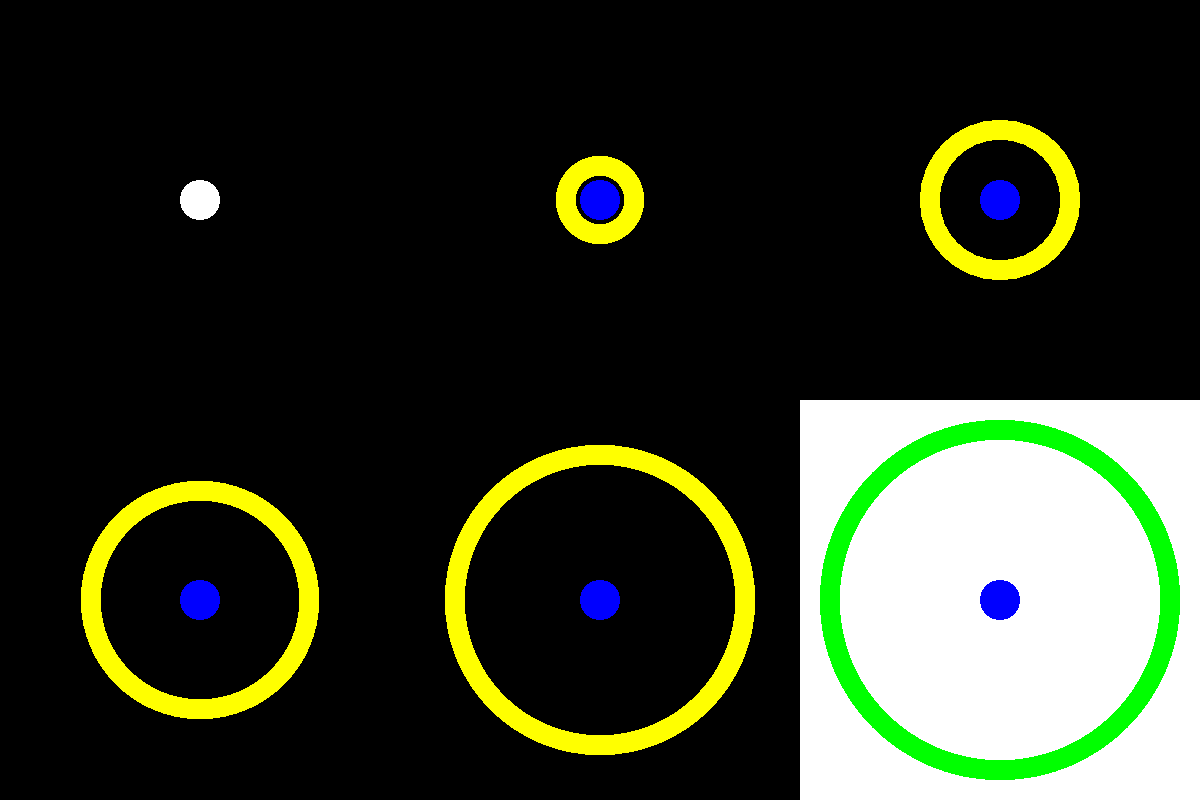
The three significant phases of the early Universe illustrated in the animation are as follows;
- Initially, energy separates into dark matter (blue) and baryonic matter (green) with photons (red) that are created by interactions between the charged particles. The combination of “green” baryonic matter with “red” photons is represented by the yellow ring (yellow being a combination of red and green).
- The baryon-photon shell expands outwards against a background that is black because there are no free photons to produce illumination.
- When the temperature cools enough for the plasma to disperse, the photons escape leaving the baryonic matter behind. The yellow ring turns green, indicating the presence of baryonic matter without any trapped photons, and the background becomes white as the freed photons are able to provide illumination.
The term “baryon acoustic oscillations” can therefore be unpicked as follows;
- It refers to baryonic matter (not dark matter).
- It refers to motion limited by interparticle energy transfer (the speed of “sound” in the plasma).
- It refers to a progressive wavefront travelling away from the dark matter core.
It took about 400,000 years before the temperature cooled sufficiently for the plasma to be replaced by combinations of protons and electrons (atoms) that were no longer opaque to photons. The shells had a radius of about 450,000 light years and the escaping photons carried with them an image of the matter distribution as it existed at that moment in time. (Figures taken from UCLA Astronomy Professor Ned Wright’s website, at https://www.astro.ucla.edu/~wright/BAO-cosmology.html.)
As the Universe expanded, two things are expected to have happened; the wavelength of the electromagnetic radiation should increase (but its image-pattern should stay the same) and the matter distributions should move farther apart (still with higher-density regions but becoming less distinct as time progressed).
The power fluctuations in the CMB are the remnants of the image created when photons were freed from the baryon plasma. If there were an observable pattern of regions with higher density across the Universe then that could confirm the second half of the picture. But this is not a trivial task because it involves identifying a subtle effect where some galaxies are closer together, in a structured way, than is the case elsewhere.
The BAO signature was detected for the first time in 2005 by two separate teams of astronomers; the 2dF Galaxy Redshift Survey (2dFGRS) in Australia and the Sloan Digital Sky Survey (SDSS) in America. The latter was led by Harvard Professor of Astronomy Daniel Eisenstein, who describes the complexity of the task as follows.
“If one region is like throwing a pebble in a pond and seeing the expanding ripple, then the Universe is like throwing a handful of gravel in pool. Nevertheless, the basic radius can still be detected statistically, and we predict that galaxies are slightly more likely to be separated by 500 million light-years than they are to be separated by 400 or 600 million light-years”. (See https://lweb.cfa.harvard.edu/~deisenst/acousticpeak/acoustic.pdf.)
There are some brilliant resources illustrating BAO principles on NASA’s Scientific Visualization Studio website at https://svs.gsfc.nasa.gov/13768. The two animated GIFs shown below are snippets that give a flavour for the main animation but I strongly recommend that you visit the website to view all the materials in full.


By combining the BAO imprint in the CMB with the angular size of observable higher-density galaxy distributions, the expansion of the Universe (the Hubble constant) can be determined without using any rungs of the distance ladder.
The radius of the baryon wavefront at the moment of decoupling (when photons were freed) has been calculated and a more-common distance between galaxies has been identified. The diameter of the higher-density regions is a standard ruler: they all originate from objects of the same initial size so differences in angular size must correlate with age (distance from Earth). This information, combined with recessional velocities obtained from redshifts, allows the Hubble constant to be determined without using a single rung of the distance ladder.

Unfortunately, the value of the Hubble constant calculated in this way is significantly different from the value obtained using the distance-ladder approach. Would more data resolve the discrepancy? The original BAO analyses were conducted using tens of thousands of galaxies, whereas the next round of data collection, currently underway using the Dark Energy Spectroscopic Instrument (DESI) aims to collect information for 30 million galaxies. (See https://perimeterinstitute.ca/news/desi-launches-five-year-quest-to-understand-the-universe for more information.)
Maybe more data will help to reduce the tension; maybe it will only reduce the uncertainty in the BAO value, making the tension worse. Whatever happens in the future, the Hubble tension is currently a troublesome problem that requires as-yet unidentified explanation.
Further reading listed below…
As well as the links given in the text, there are several more that are worth exploring. In particular, Michael Richmond, Professor of Astronomy at Rochester Institute of Technology, has created a really nice summary that is available at http://spiff.rit.edu/classes/phys372/lectures/tension/tension.html but note this is an http site, not https, so some browsers may not load it.
A technical overview is available at https://physicstoday.aip.org/features/baryon-acoustic-oscillations-a-cosmological-ruler and much greater detail is available on the pages written by Harvard Professor of Astronomy Daniel Eisenstein, whose group continues to use BAOs “to measure the cosmic distance scale and thereby probe the acceleration of the expansion history of the Universe and the properties of dark energy”. To find out more, visit https://deisenstein.scholars.harvard.edu/book/baryon-acoustic-oscillations.
For nice explanation that includes the non-constant nature of the Hubble constant indicated by the accelerating expansion of the Universe, see NASA’s Nancy Grace Roman Space Telescope page at https://science.nasa.gov/mission/roman-space-telescope/baryon-acoustic-oscillations/.
As of August 2026, there is an easy-to-read summary of some highlights in current cosmological research, including work being undertaken by young astrophysicists and the ways in which different fields of activity link together, on the Perimeter Institute website, at https://perimeterinstitute.ca/news/future-cosmology.
Finally, Wikipedia offers a good collection of information and references related to the Hubble constant as part of a broader series on Physical Cosmology (see https://en.wikipedia.org/wiki/Hubble%27s_law and https://en.wikipedia.org/wiki/Baryon_acoustic_oscillations).


