Exponential changes

Imagine an empty tube train (metro, if you prefer) pulling into a crowded station. When the doors open, people surge forward and the carriage starts to fill very quickly. As the number of people in the carriage increases, the number of remaining spaces decreases and the rate at which further people can board also decreases. After a while, the carriage will be so full that more people will only be able to board if those inside redistribute themselves to occupy spaces away from the doors. The rate of boarding will drop to a mere trickle until nobody more can join the carriage. The doors then close and the train leaves the station.

Although I have never collected the actual numbers, the situation described above is very likely to be an example of exponential change. The definition of an exponential change is one where the quantity varies by an amount that depends on its current value.

A quantity that doubles every day would be a good example of an exponential growth. Bacterial coverage on a nutrient agar plate can follow exponential growth in its early stages but the area of the plate is finite so the growth will slow and must eventually stop. Similarly, the number of passengers occupying a crowded carriage increases very quickly at first then slows down as maximum occupancy is approached.

You may notice that I initially described the train carriage with reference to the number of remaining spaces, which drops to zero, whereas I have now mentioned the number of passengers, which increases to a maximum value. These are the two general cases for exponential changes and are shown in the graphs below for some general quantity, A.

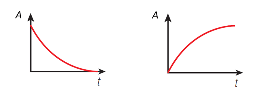
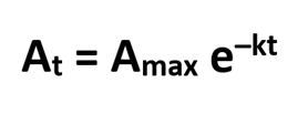
For an exponential decrease (as in the left-hand graph) the general equation looks like this;

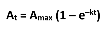
Conversely, if there is an exponential increase towards a limiting value (as in the right-hand graph) the general equation takes the form;

In both cases;

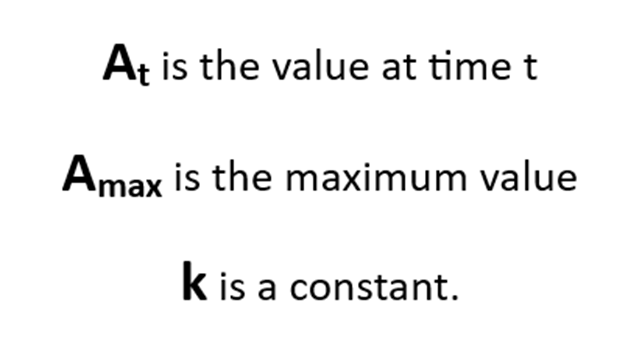
Importantly, in the first equation the maximum value (A_max) occurs at time zero and can therefore be measured before any subsequent changes take place. But in the second equation the maximum value is achieved after an “infinite” amount of time yet is required in calculations that apply to earlier instances, which means a predicted value has to be used. For this reason, if there is the option to use either form, the first equation is often preferable.

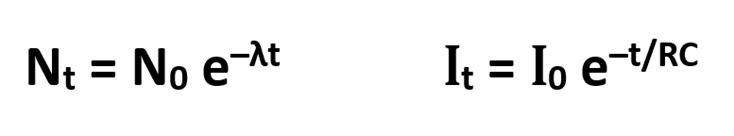
The constant in the equation, k, is determined by the situation to which the equation applies. In the case of radioactive decay, the constant is related to the probability of decay, which in turn determines the number of nuclei that will decay in a given time. In the case of current flow when a capacitor is either charging or discharging, the constant is equal to the reciprocal of the product of the circuit’s capacitance and resistance.

The specific equations for these two applications are given below;

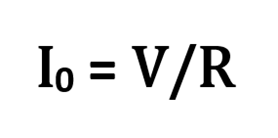
In the capacitor case, we can go further and predict (as well as measure) the initial maximum current, which will be equal to the supply voltage divided by the circuit resistance;

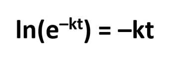
To analyse these equations it is useful to move time out of the power term. This can be done using natural logarithms by exploiting the fact that the natural logarithm of e raised to a power is simply equal to the power itself. Expressed algebraically, this means;

So if we rearrange the general equation then take natural logs, we can get;

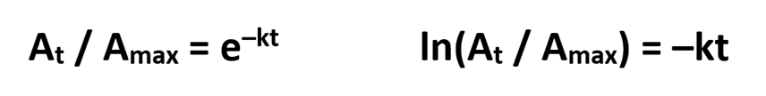
We can then use the fact that a division within a logarithmic expression is the same as subtracting the two individual logarithms;

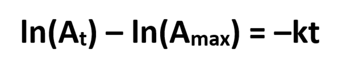
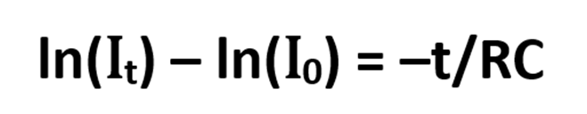
Reverting back to the specific case for current flow when a capacitor is charging or discharging, we can write;

and rearrange to give a y=mx+c form that allows linear analysis;

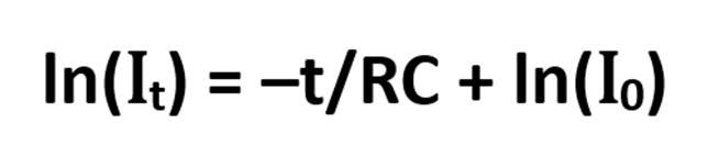
where the y-intercept is the natural logarithm of the maximum current, I₀, which is itself equal to V/R, and the gradient is the negative reciprocal of the time constant, RC.