It is reasonable to expect a lamp’s apparent brightness to decrease with increasing distance from the source but what is the best way to determine the nature of the variation? Although there’s a theoretical answer that applies to all electromagnetic waves, based on the inverse-square law, it is important to be able to carry out an experimental investigation to confirm (or maybe even reject) the expected relationship.
The experiment is easily done using a visible-light source but the same principles also apply to the fall-off of gamma radiation with distance from a radioactive source, which is a required practical in the AQA A-level Physics course.
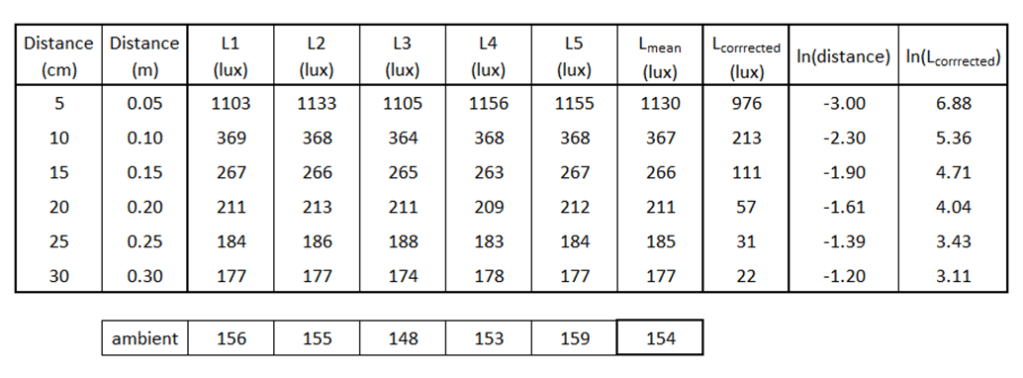
Several of my students recently carried-out the visual-light investigation and the two sets of data used here were collected during that exercise. The raw data from the first student are shown in the table below;
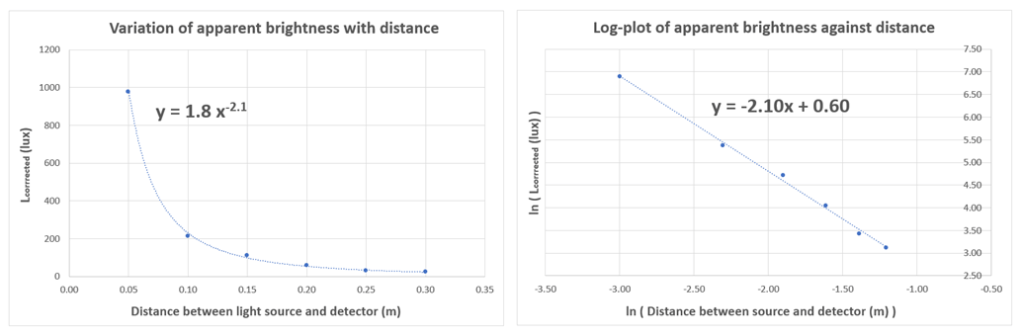
A scatter plot of distance (in metres) against corrected mean light measurement (in lux) reveals an inverse-type pattern where there is a non-linear decrease in illuminance with increasing distance. The best-fit curve corresponds to a power of –2.1 and produces a very close-fitting line, as shown on the left-hand graph below. The right-hand graph is a scatter plot of the logarithms of the values and reveals a good straight-line fit with a gradient of –2.1, which is consistent with the power fit. Both plots were created using Microsoft Excel.
The second student’s data covered a wider range of distances with a similar estimate of the ambient lighting level but the data suggest the actual background illuminance in this case was higher than the stated value. This can be seen in the left-hand graph below, where there is a clearly-indicated plateau at about 240 lux even after correcting for the ambient light level. Unlike in the first student’s graph, the power-law relationship is not an especially good fit for the data plotted.
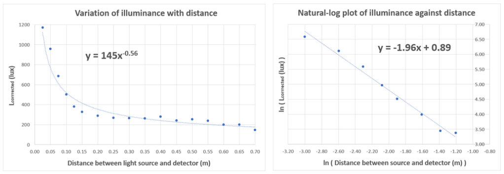
Confining the second student’s data to the same range as was used by the first student, and using a logarithmic plot, produces a result that is generally consistent with the previous findings. The right-hand graph reveals a good straight-line fit with a gradient of –1.96 and a constant of proportionality equal to 2.4 (e0.89).
Overall, the two sets of data offer reasonable support for the theoretical inverse-square model and are accompanied by similar values for the constant of proportionality (1.8 and 2.4).
The constant of proportionality is indicative of the abolute brightness (luminosity) of the light source. Common LEDs generally transfer about 80 lumen-per-watt with a maximum current of about 100 mA: the apparatus used had a 3 V power supply (two AA cells) so was probably rated at about 0.3 W and therefore ought to have produced about 24 lumens. This is about an order of magnitude greater than the values obtained from the graphs but there is another factor that hasn’t been taken into account.
The inverse-square law stems from a model that involves the surface area of spheres at different distances. Specifically, a sphere that has twice the radius of another sphere will have four times the area. This means the light emitted from a source at the centre of the larger sphere will be spread over four times the area of the smaller sphere and is therefore four times dimmer.
This is enough to explain the proportional relationship but to be more complete we should include a factor for the luminosity of the light source AND a factor of 4π that originates from the spherical model used. When these components are included, the proportional relationship shown below on the left can be transformed via a general equation (centre) into the specific equality shown on the right.
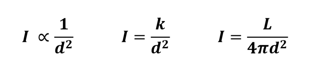
The constant of proportionality is therefore equal to L/4π, where L is the luminosity of the light source, which we have estimated to be about 24 lumens. When this figure is divided by 4π, we get a value of 1.9, which sits nicely within the range provided by the two sets of experimental data.
In conclusion, both sets of data support the inverse-square law as a general relationship linking apparent brightness (illuminance) with distance from the light source. More specifically, the constant of proportionality obtained in the two experiments is consistent with the estimated characteristics of the LED light source used.
All of which sounds great but there is still one thing left unchecked: is the illumination pattern of an LED genuinely spherical? The short answer is “no”: LEDs cannot radiate light behind the emitting surface. We then have to ask whether they genuinely behave as if they radiated light in all directions…
That will be the topic for another post but, in the meantime, it is important to note that having results that support a preconceived theory does not prove the theory is right. There is a pitfall in all experimental science known as “confirmation bias”: this is where an experiment finds the expected results but does not check whether the expected results are caused by the suggested theory.
The best science looks for ways to challenge theories, not simply to confirm them.


