Charging a Capacitor (analysis)

Changes in charge, current and potential difference during the charging and discharging of a capacitor are all exponential-type behaviours. Specifically, the current that transfers charge to or from a capacitor (during charging or discharging respectively) is always greatest at first and declines to zero as time increases. During discharging, the charge loss and the drop in potential difference also show exponential decay, declining from an initial maximum value to zero. But during charging, the charge and potential difference both increase to a finite maximum value.

The general equations for these two behaviours are shown below, where A is the appropriate quantity, as listed;

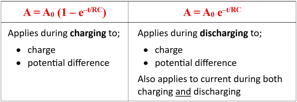
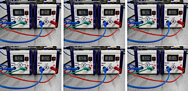
These relationships can be checked experimentally by recording values for the appropriate quantities at different times during charging or discharging. In practice, this can be quite tricky as it involves observing multiple values simultaneously. Data-logging is the ideal solution but it is also possible to record the displayed values photographically, using video or sequences of still images.

Plotting the recorded values for potential difference and current obtained from the full picture sequence gives the two graphs shown below;

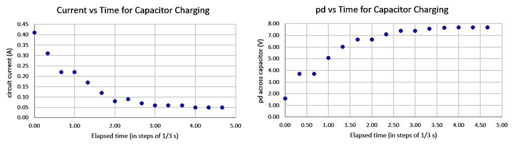
Although the curves indicate the expected trends, the data are not convincing. In particular, the current curve does not reach zero but tends to a finite value that is likely to be around 0.04 A. It is therefore useful to limit the data to the time range where there is the clearest rate of change, for which the cut-off is at about 3.0 s.

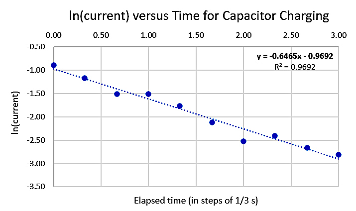
Bearing in mind that the current is expected to show an exponential decay ( I = I₀ e^–t/RC ) we would expect that plotting the natural logarithm of the current against time will give a straight line ( lnI = ln(I₀) – t/RC ). This is illustrated below.

Analysing the data for potential difference is slightly more complicated but can be simplified by rearranging the usual equation into the form 1 – V/V₀ = e^–t/RC then converting to natural logarithms and plotting ln(1 – V/V₀) against time. In order to use this approach, it is necessary to assume a final value for the maximum potential difference: in this case, the limiting value has been estimated to be 7.7 V based on the available data.

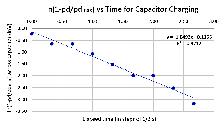
Comparing the equations for the line-of-best-fit in each graph, we can see that the time constant seems to vary significantly, from 0.95 s to 1.5 s. These values can be compared with the expected value based on the capacitor and resistor used, which had values of 58 mF and 20 Ω respectively. The theoretical value for RC is therefore 1.2 s, which exactly matches the midpoint (mean) of the two measured values.

It is also worth noting that the value for ln(I₀) obtained from the current graph suggests an initial current of 0.38 A. This can be compared with the expected maximum current according to Ohm’s law using the circuit’s resistance (20 Ω) and the assumed maximum potential difference (7.7 V) which combine to give a current of 0.385 A. The high level of consistency that exists between the calculated current and the value obtained by graphical analysis provides further confidence in the original data and the analysis methods used.