Uncertainties and Error Bars

Measurements are always uncertain: there is no such thing as a perfectly precise measurement. At the very least, the instrument used will limit the precision of the value but in many cases other factors can introduce even greater variability. It is always the greater of these two numbers (the resolution of the instrument and variability in the readings) that is quoted as the final uncertainty.

A few examples will help to explain how this works in practice.

In an experiment to investigate the resistance characteristics of a filament lamp, it is necessary to collect data for both the potential difference across the lamp and the current flowing through it. The potential difference and current values are then combined to calculate resistance ( R = V / I ).

Let’s say that each measurement is taken five times to check for repeatability. The mean for each set of five values is then calculated and the uncertainty will be determined as +/- half the range of the results (or the resolution of the meter used, if that is greater than the uncertainty calculated using the range).

An example set of results is shown below;

The mean, range and uncertainty due to the range for these results are shown below;

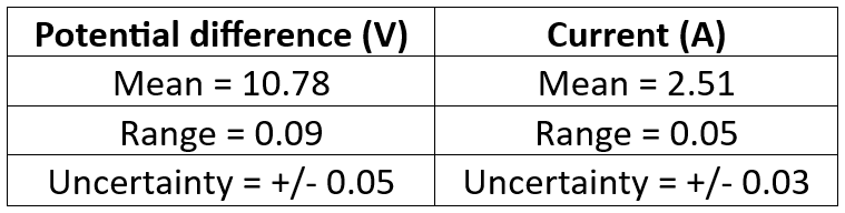
The meters used for these measurements both had a resolution of +/- 0.01, so the final uncertainty in the measurements can never be less than +/- 0.01. Similarly, the instrument resolution makes it inappropriate to state the uncertainty to more than two decimal places, which is why the final values have been rounded.

When plotting a graph, the error bars extend a distance from the plotted point that is equal to the uncertainty. The plot for the potential difference will therefore have its “x” at 10.78 and error bars that end on 10.73 (10.78 – 0.05) and 10.83 (10.78 + 0.05).

In order to calculate the resistance of the filament lamp, we must divide the mean potential difference by the mean current. To calculate the uncertainty in the resistance, we must sum the percentage uncertainties in the two means.

The resistance calculation is straightforward and gives a value of 4.29 Ω.

The steps involved in calculating the resistance’s uncertainty are shown in the table below;

It is the absolute uncertainty that is used to plot the error bars. Therefore, the plot for the resistance value will have its “x” at 4.29 with errors bars that end on 4.22 (4.29 – 0.07) and 4.36 (4.29 + 0.07).

Now let’s look at a second set of results;

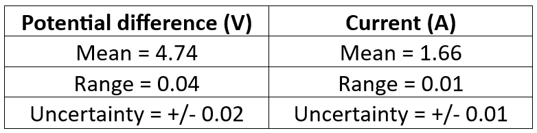
In this case, halving the range for the current would suggest an uncertainty of +/- 0.005 but, as has already been pointed out, it would be wrong to state an uncertainty value smaller than the meter’s limiting resolution of +/- 0.01.

In this case, the plot for the potential difference will have its “x” on 4.74 and error bars that terminate at 4.72 and 4.76. The mean resistance works out to be 2.86 Ω but can you use the same process as before to calculate the uncertainty in the resistance for this set of data? According to my calculations, the errors bars end at 2.83 and 2.89 (+/- 0.03).

In many cases, the error bars will be very short and could even be too small to plot but you still need to determine the final uncertainty in all values to guard against cases where the error bars can have a significant effect when drawing the optimum line-of-best fit.

Finally, I should add that this approach is specifically aimed at the expectations of the AQA A-Level Physics examination: it is not strictly correct in a wider context. For a more thorough treatment of uncertainties, I strongly recommend a short and very readable booklet issued by the National Physical Laboratory that can be downloaded from https://www.npl.co.uk/resources/gpgs/beginners-guide-measurement-uncertainty-gpg11