Hypothesis and Analysis

When carrying out a practical investigation it is always helpful to know what sorts of results are expected. In other words, before starting an experiment it is a good idea to consider what theory tells us should be the outcome.

The predicted findings form the basis of an hypothesis, which is developed by considering an ideal experiment and is tested by comparing the actual results with what would be expected in theory.

If this sounds very circular, it is! Most experiments are tests of existing theories and do not set out to discover anything truly new but rather are extensions of what is already known or believed to be true.

One of the current A-Level practicals involves students determining the resistivity of a wire and a selection of wires, made from different materials, is provided. Which wire will be the best choice? Maybe the prettiest one? Manganin looks a bit like gold; copper has a lovely rich colour; nichrome is nice and shiny; constantan looks rather dull by comparison.

Obviously, physical appearance isn’t a good basis for selecting the wire to use. In fact, given that the purpose of the experiment is to determine the wire’s resistivity, it makes sense to start by researching the expected values in order to decide how easy they will be to measure. It also makes sense to discover how sensitive is each wire’s resistivity to changes in temperature.

Good sources of information relating to engineering materials and applications include Engineering Toolbox (https://www.engineeringtoolbox.com/) and the Space Materials database (https://www.spacematdb.com/spacemat/). These two references were used to compile the table of data given below.

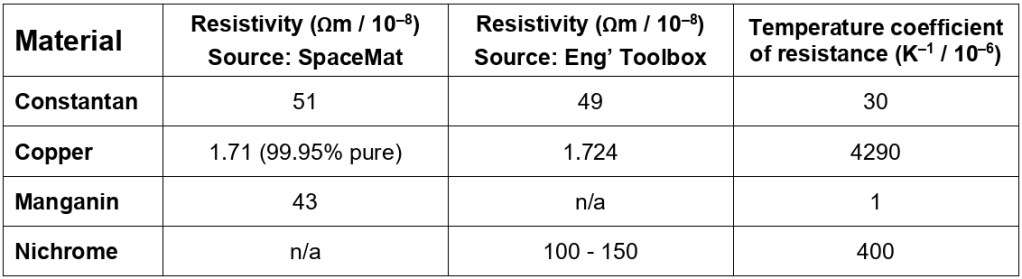
Given these characteristics, it is easy to eliminate copper (why?) but a case could be made for choosing any of the others. Although the wire diameter will also have to be taken into account when designing the experiment and analysing the results, it is important to be able to rationalise whichever material is chosen as well as the selected wire diameter (if different gauges are available).

At the other end of the investigation there will be a set of results to be analysed. When determining the resistivity of a wire, these will be data that correlate wire length with calculated resistance, determined by measuring the potential difference across the wire and the current that flows through it.

The resistance must be calculated for each pair of current and potential difference values: this method is much better than averaging all the currents and the potential differences at one length then dividing the two average values to give an average resistance.

Why are multiple resistances required for each wire length? Because the individual values of resistance will reveal the uncertainty in the measurements, which is separate from (and often much greater than) the uncertainty in each individual reading, as determined by the precision of the measuring instruments used.

For example, if five readings were taken for current and potential difference at one particular length of wire, they might all produce identical values for resistance (1.23, 1.23, 1.23, 1.23, 1.23) or they might exhibit some scatter (1.24, 1.26, 1.23, 1.20, 1.22). These two data sets have the same instrument uncertainty (+/- 0.005) and the same mean but they are differentiated by their range, which is the difference between the largest value and the smallest value.

The uncertainty in the resistance can be taken to be +/- half the range. For the first set of results, the uncertainty appears to be zero but is actually limited by the precision of the meters used whereas the uncertainty in the second set of results has a calculable value, which is +/- 0.03 (half of 1.26 – 1.20).

To explore the analysis in more detail, let us consider a certain experiment in which the calculated resistances, mean values and uncertainties, were as follows and generate an intial graph as shown below.

The line of best fit does not intercept the origin but the discrepancy is very small (0.09) and is likely to be accommodated by the scatter of values within each data set. As it happens, forcing a zero intercept does not change the R-squared value (correlation coefficient) of the line to any significant degree.

Given that a directly proportional relationship is expected in this experiment, and the data appear to allow such adjustment, it could be valid to force a zero intercept even though this is generally considered to be poor practice. The zero-intercept graph is shown below.

Neither of the graphs indicates the accuracy of each value and therefore the likely accuracy of the calculated resistivity. One way to indicate accuracy is by using error bars, which for small sample sizes can simply mark the highest and lowest value of the resistance readings.

The error bars (or the results that mark their ends) can then be used to plot the shallowest and steepest lines of best fit that will go through the limits of the bars rather than through the mean values. The two graphs shown below have been plotted in this way and their gradients indicate the range of final values allowed by the calculated resistances given in the table earlier.

Analysis of this particular experiment is therefore likely to involve using the gradient for the mean-resistance line, which is 4.87 for the zero-intercept version, together with the steepest allowable gradients; 4.86 and 4.90 respectively. It is worth noting that the allowable gradients are not symmetric around the mean – and that there is no requirement for this to be the case since the non-mean gradients are determined by the scatter of the calculated values, which are not necessarily symmetrical about the mean.

The gradient for the unadjusted plot (4.75) could also be used but in this case the value of the non-zero intercept would need to be discussed.