Measuring Speed

This is the third part of a mini-series looking at motion and here we’ll be considering different ways to measure speed as well as some common sources of error.

In theory, speed is easy; we just need a distance (measured using a ruler, for example) and a time (probably measured using a stopwatch but ideally using an electronic system).

The choice of distance measurement instrument depends on the scale of distance that is to be measured: in the lab, a metre rule will generally be most appropriate.

Some years ago there was an examination question that had students pacing out the distance between lamp-posts to measure the speed of a vehicle. This was clearly very inaccurate and marks were awarded for suggesting an appropriate improvement to the method used. A good answer would have been to suggest using a tape measure or a trundle wheel – but not measuring the length of one pace and multiplying up (because stride length could still vary).

Remember the procedure for determining the uncertainty in measurements: if a trundle wheel is marked in 10 cm divisions then you can only measure to the nearest 10 cm (you should not attempt to estimate the distance within an unmarked range) and the resolution of your measurement is therefore +/- 5 cm (half of the smallest marked division).

Using a stopwatch brings its own source of error in the form of human reaction time. Typical human reactions are around 0.1 s to 0.2 s but they are random errors that are likely to be slightly different for every measurement, causing the results to be imprecise (vary for each reading). Random errors are best handled by taking repeated readings and, after eliminating any obvious anomalies, calculating the mean average.

Using a carefully-measured distance and a mean time we can determine the average speed of an object by dividing the distance by the time;

Note that the result is an “average” speed because the speed may have varied slightly across the measured distance, not because we used an average time.

To avoid random errors (human reaction time) it is better to use an electronic timing system. This could be a digital timer that is started when the object passes through one light-gate and stops when the object passes through a second light-gate. Repeated measurements should always give the same time interval (precise results) because the electronic system is very reliable (does not have any sources of random error). If the times vary, then the actual motion of the object is changing, perhaps due to the object not always following the same path. As usual, repeating the measurements, eliminating any obvious anomalies then calculating the mean time will be the correct way to proceed.

It’s worth adding that some light-gates contain both the start beam and the stop beam in one housing: as such they are able to give a speed read-out without the user having to do any calculations. This type of light-gate is useful for determining acceleration, which will be discussed in the next article.

Instead of using light-gates, a pair of pictures can be used to determine the speed of an object. In this method, a second picture is taken a certain amount of time after the first, and the distance moved by the object can be measured if the same scale (such as a metre rule) is included in both pictures. Let’s analyse the two pictures shown below as an example.

The camera was set to record pictures at three frames-per-second (3 fps) but I also included an electronic stopwatch in the pictures to ensure that this figure was accurate. I did repeated readings and the time interval was always 0.32 s. You probably can’t read the time figures on the scaled-down pictures shown here: more importantly, you can’t read the distance scale either, so let’s look at some enlarged sections of the two images.

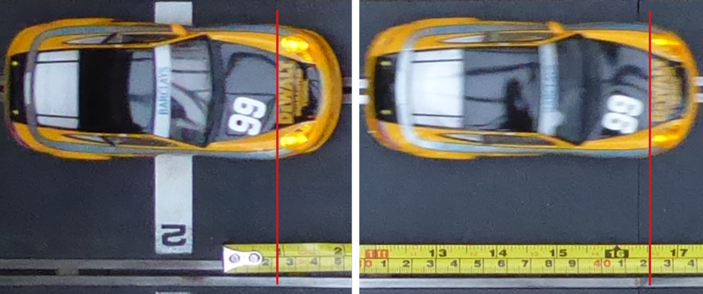
The distance scale is not clearly resolved here but it is just about possible to see the millimetre markings in the original pictures. Rather than measuring the position of the front of the model car, which is a curve and rather indistinct due to blurring, I have chosen to mark a clearer part of the car’s bodywork, shown with red lines on both images. The red line falls at 2.2 cm in the first picture and 42.0 cm in the second picture. This gives a distance moved of 39.8 cm (0.398 m). The time taken was 0.32 s so the speed of the model car in this experiment was;

We could have kept the distance in centimetres, in which case the speed would have been 124 cm/s. Note here the importance of including the appropriate units! The two answers (1.24 and 124) are both correct but only when they are accompanied by their corresponding units. It is also worth noting that, owing to the blurring, it would be acceptable (and probably advisable) to quote the final answer to just two significant figures; giving 1.2 m/s or 120 cm/s,

In the next article we will progress from measuring speed to measuring acceleration.