Kinetic Theory

Scientific theories are constructs (models) that we use to explain our observations. They are different from scientific laws, which are rules that have to be obeyed and which can be applied across a wide variety of situations. The best known example is the Big Bang Theory but we’ll be looking at a theory that relates to the behaviour of gases.

I have touched on some of this in a previous post, Absolute Zero, but in many ways it makes more sense to read the current article before you read about absolute zero (even though I wrote them the other way around).

The origins of Kinetic Theory are rooted in the idea that the energy stored in a substance, which varies with its temperature, is due to the movement of its particles. The hotter a substance is, the more energy each particle will carry. Given that the energy of each particle is exhibited as movement, the type of energy that applies here is kinetic energy.

And that’s the essence of Kinetic Theory; the temperature of a substance is due to the kinetic energy of its particles.

If the substance changes state, there will also be a change in potential energy but if we keep to one state alone then the temperature of a substance is due only to the kinetic energy of its particles.

There is a whole load of really interesting stuff that stems from this basic idea, including a contribution from Albert Einstein, but in our course we focus on its application to gases. (In fact we’re further confining ourselves to “ideal gases”, where each gas particle is an independent entity with zero volume: this may sound impossible but it works really well.)

There is a fantastic online animation that you can use to explore the movement of gas particles at different temperatures. The animation is available at https://falstad.com/gas/ and a screen-grab (without the essential animation, of course) is shown below.

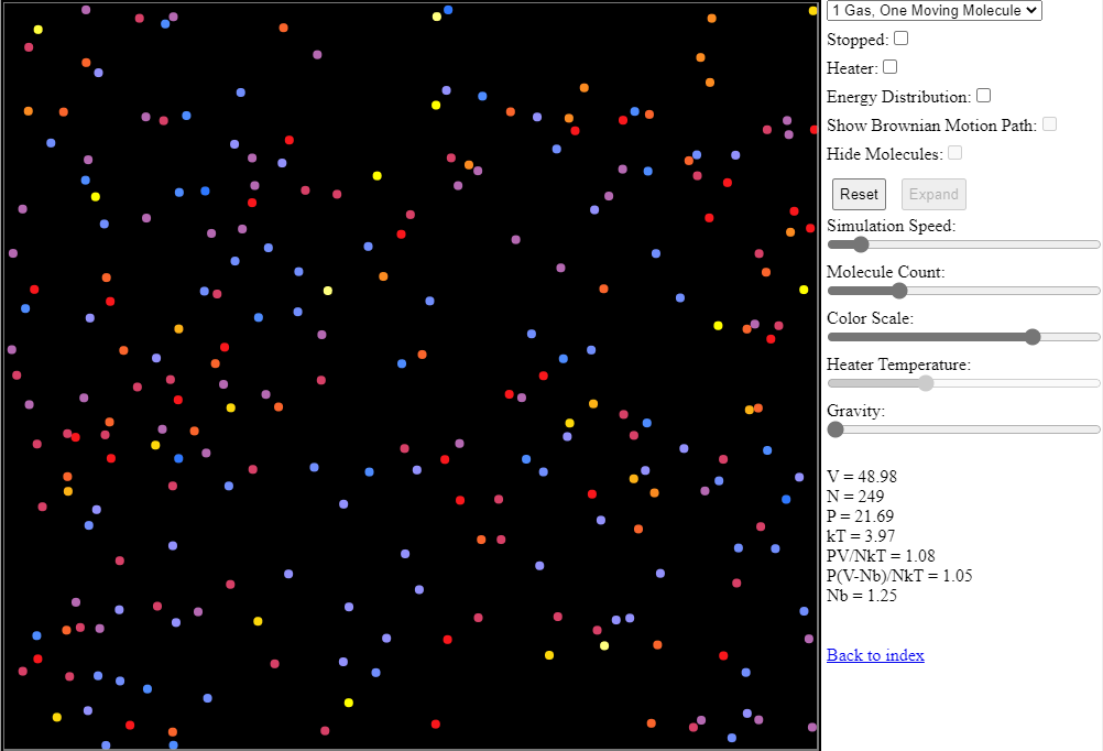
To understand the animation better, move the Molecule Count slider all the way to the left (just one particle) then move it up slowly to see what happens as more particles are introduced. You should notice that the speeds of the particles vary – and there is a useful histogram at the bottom of the screen that shows the distribution of these speeds for all the particles. In keeping with the traditional representations of temperature, blue particles have lower temperature (energy), red particles have medium temperature (energy) and yellow/white particles have the highest temperature (energy).

In our course we overlook the fact that particles have a range of different speeds but it’s good to know this is the case (as evaporation is very hard to explain otherwise).

Let’s look at the collisions that occur between the gas particles and the walls of the container (the sides of the box in the animation). It is obvious that the particles rebound but can we be more exact than that? If you watch closely you will see the only thing that changes during the rebound is the component of the particle’s movement that is perpendicular (at right angles) to the container’s surface. In other words, the path of a rebounding particle looks the same as a light ray reflecting from a plane mirror. (Don’t take the analogy too far: this does not prove light rays are simply streams of particles!)

To push the particle back, the surface must exert a force on the particle. Given that the only change in movement is perpendicular to the surface, the force must also be perpendicular to the surface.

Of course, surfaces don’t create forces on their own: the force from the surface is actually a reaction force caused by the impact of the particle, which in turn arises from the particle’s change in momentum. For now we will simply call this a forward momentum (towards the surface) becoming a backward momentum (away from the surface). Momentum, like force, is a vector quantity. Note that momentum and force are not the same thing: the connection is simply that a force is required to change the momentum of an object.

Linking back to our original idea that the temperature of a substance (gas in this case) is a measure of the overall kinetic energy of its particles, we can now go on to link temperature to pressure.

To do this, we use the following steps;

• link temperature to kinetic energy (greater temperature means more kinetic energy)
• link kinetic energy to speed (greater kinetic energy means more speed)
• link speed to momentum (greater speed means more momentum)
• link the conversion between forward and backward momentum to the force that is exerted on the container surface
• link the force exerted on the surface to pressure (force divided by area)

This means that as the temperature of a gas increases, so does the pressure it creates on the walls of the container enclosing it. And the force that causes this pressure acts perpendicular (at right angles) to the surface in an outwards direction. Why outwards? Because the gas is trying to “escape” from the container. These are key facts that you need to know!

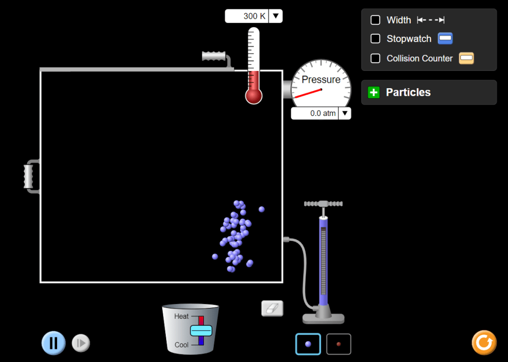
To explore this in more detail, I recommend using the gas properties animation in the online PhET suite of simulations, which you can find at https://phet.colorado.edu/sims/html/gas-properties/latest/gas-properties_en.html. There’s lots to explore so let me give you a few suggestions. Before you start, make sure that you’re in the Explore module (the link above should take you straight there).

Start by clicking on the pump handle; drag it up then lower it down again to push gas into the container. Notice that the pressure stays at zero until particles start colliding with the container’s walls. (A screen-grab of this brief state is shown below.)

Drag the Heat/Cool slider up to warm the gas: the temperature increases (you can switch to degrees Celsius using the drop-down arrow beside the display) and the speed of the particles also increases. This in turn causes the pressure to increase.

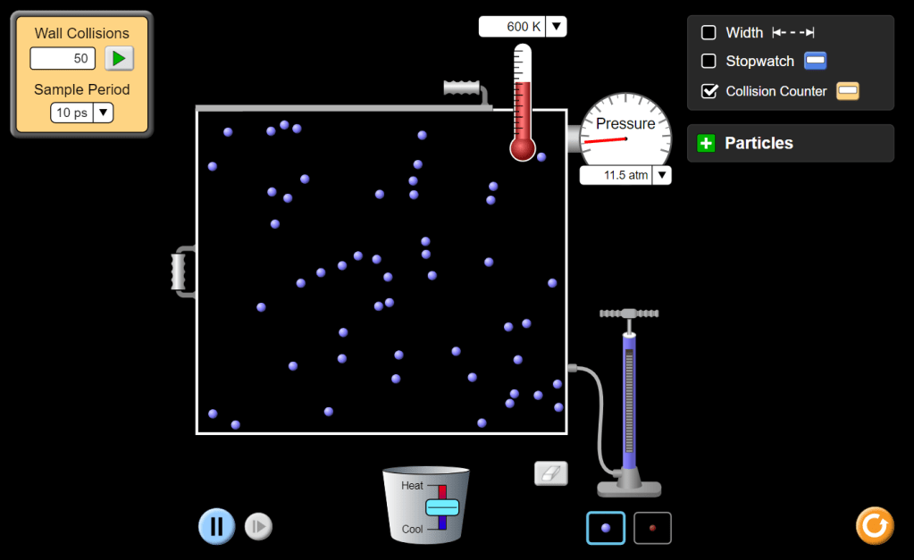
Finally, turn on the collision counter and observe the collision rate for various temperatures. Repeat your measurements (of course) because collisions are random events and their number will vary so you’ll need to take that into account if you attempt any sort of analysis (This is beyond the scope of our course but it’s a good activity for those who are keen to learn more. If you’re tempted, then collect data for the number of collisions in a fixed time interval for different temperatures: plot a graph and see what you get.) A representative result for 600 Kelvin is shown in the screen-grab below.

Footnote: I am acutely aware that I’ve used the terms kinetic energy and momentum without any careful explanation and I hope you will simply accept this for now. We’ll look much more closely at these two properties of moving objects in another article.