How to determine voltages inside a resistor network

Resistor networks sometimes look scary but they can be solved by taking things one step at a time and applying basic circuit rules. The rules concerned are the calculations for combining series and parallel resistors, together with Kirchoff’s two laws for circuits.

To combine resistors, we add their values if they are arranged in series and we take the reciprocal of the sum of their reciprocals if they are in parallel.

Now let’s remind ourselves about Kirchoff’s circuit laws;

Kirchoff’s first law is essentially a statement about the conservation of charge whereas his second law is a statement about the conservation of energy: energy out (sum of pds) equals energy in (sum of EMFs).

So let’s use these tools to determine the value of a potential difference across part of a resistor network. What is the reading on the voltmeter in the circuit below?

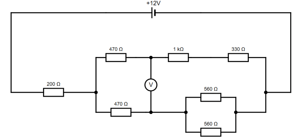
First, we will simplify the circuit as much as possible in order to work out the potential difference across the 200 Ω resistor and across the whole of the complex resistor network. Forget about the voltmeter for now!

• Step 1 is to reduce the two 560 Ω resistors in the small parallel network to one 280 Ω resistor (using the rule for combining parallel resistors).

• Step 2 is to turn each arm of the large parallel network into single resistors of values 1800 Ω and 750 Ω (using the rule for combining series resistors).

• Step 3 is to use the rule for combining parallel resistors to reduce the two remaining resistors in the large parallel network to a single resistor of value 529 Ω, which will then form a series combination with the original 200 Ω resistor.

These three stages of simplification are represented in the diagrams below.

The final simplified circuit comprises just two resistors in series, 200 Ω and 529 Ω, giving a total resistance of 729 Ω. The EMF of the cell will be divided across the two resistors in the ratio of their individual resistances.

• The potential difference across the 200 Ω resistor is given by (200/729) x 12 = 3.29 V.

• The potential difference across the 529 Ω resistor is given by (529/729) x 12 = 8.71 V.

To check we haven’t made a mistake, it’s worth noting that the sum of these two potential differences is equal to the EMF of the cell, as required by Kirchoff’s second law.

Now we can return to the first stage of simplification knowing how the overall voltages are divided up. We can completely ignore the 3.29 V that is across the 200 Ω resistor. In fact, we can ignore that part of the circuit entirely and imagine the power supply is delivering only the 8.71 V provided to the parallel network. This arrangement can be drawn as shown below.

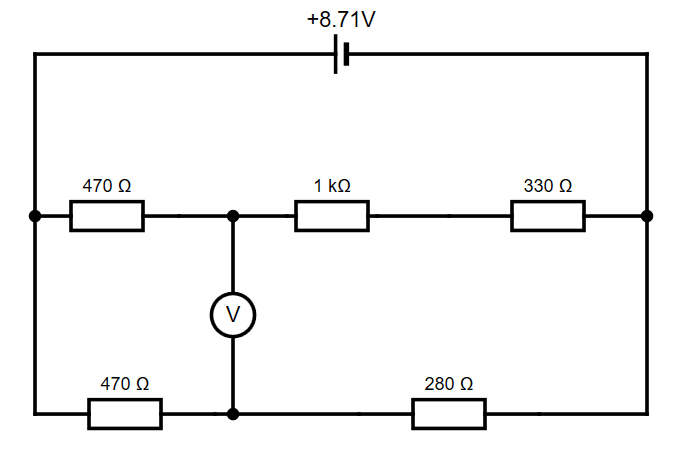
It may not be obvious but we are nearly there as we only need to realise that each branch of the parallel network is connected directly to the power supply and the EMF of 8.71 V is therefore divided across the resistors in each branch independently.

In the case of the lower branch, the total resistance is 750 Ω so the potential difference across the 470 Ω resistor is (470/750) x 8.71 = 5.46 V. The point where the voltmeter connects into the lower branch will therefore be at 3.25 V (8.71 – 5.46) relative to the zero side of the power supply.

In the upper branch, the total resistance is 1800 Ω and this means the potential difference across the 470 Ω resistor will be (470/1800) x 8.71 = 2.27 V. The point where the voltmeter connects into the upper branch will therefore be at 6.44 V (8.71 – 2.27) relative to the zero side of the power supply.

Finally, the difference between the potentials at these two points will be equal to the voltage displayed on the voltmeter. The answer to the question is therefore 3.19 V

If you want to be picky, I cheated slightly at the end by talking about the potential at a point instead of potential differences between two points but if you read carefully you will note that the points were both specified relative to the same reference (the zero side of the power supply) so they were in fact potential differences.

FOOTNOTE: All the diagrams in this post were created using Sam Fisher’s excellent (and free) Circuit Diagram software, which is available online at https://www.circuit-diagram.org/