Paper 3a, Q3 walk-through

This post completes an explanation given to my current Y13 students, which was unfinished at the end of our lesson. It relates to the second half of Q3 in Paper 3a for the AQA A-Level Physics examination of June 2023. You can download a copy of the complete paper here.

To solve Q3.4 you must first ensure that you understand the diagram given in Figure 10, which is a two-coil arrangement echoing the single-coil version shown earlier in the paper as Figures 7a and 7b. These illustrations are shown together below.

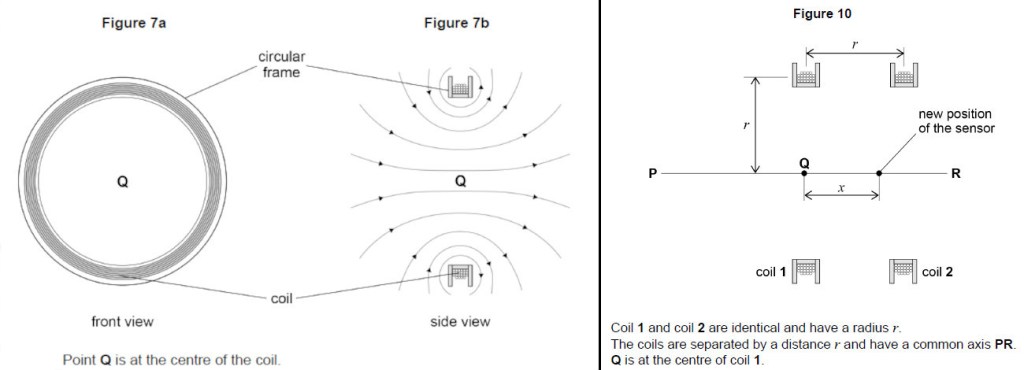
The important thing about Figure 10 is it shows the path of a sensor that is moved along the common axis of the coils, from P via Q to R. This is done twice; first with a current flowing only in Coil 1 and then with the same current flowing only in Coil 2.

Figure 11 (shown below) plots the change in magnetic flux density as the sensor’s position is varied during the two experiments. In both cases we expect the magnetic flux density to be strongest when the sensor is at the centre of the coil that is switched on.

The distance between the two peaks, measured on the x-axis in Figure 11, equals the distance between the two coils, and is also equal to the radius of each coil, as shown in Figure 10.

Having understood the information contained in Figure 10 and Figure 11, we are now in a position to answer Q3.4, which asks for the value of the ratio of x_0.5 divided by r, where x_0.5 is defined as the displacement (vector distance) at which the value of the magnetic flux density falls to half of its value at Q.

First we must find the value of the magnetic flux density at Q (the maximum value). This is 0.665 mT. Then we need to halve the maximum value, giving 0.3325 mT, and check the graph to find the location (distance from Q, indicated on the x-axis) corresponding to this new value. We are only interested in the solid line on the graph because that is the curve that relates to Experiment 1, as specified in the question.

I read the displacement to be 52 mm (the mark scheme allows 50 – 55 mm).

To find the value for r, we check the displacement between the two peaks in Figure 11, as the two peaks occur at the centres of each coil. I made this value 68 mm (the mark scheme allows 67 – 69 mm).

Therefore, the value of the ratio, x_0.5 divided by r, is equal to 52 / 68, giving 0.78. The mark scheme allows values in the range 0.73 to 0.81. Note that here are no units as this value is simply a ratio.

Q3.5 concerns a third experiment in which both coils are switched on at the same time. We are told that the magnetic flux density has a constant maximum value across the displacement range from r/4 to 3r/4: we have to calculate what that constant value is.

Using r = 68 (from the previous part of this question) my values for r/4 and 3r/4 were 17 mm and 51 mm respectively. We can use Figure 11 to add the values of magnetic flux density for two curves at each of these locations, checking that they give the same total, and that is our answer.

I got a quicker answer by noticing that the curves cross within the specified range so the maximum magnetic flux density is simply equal to twice the value where the curves cross. This occurs at 0.475 mT, giving a maximum magnetic flux density of 0.95 mT. The mark scheme ranks answers according to their accuracy;  answers in the range 0.91 – 0.99 mT score just one mark whereas answers in the range 0.93 – 0.97 mT score both marks.

Q3.6 asks you to state two characteristics of the field lines “in this region”. You need to realise that the question is referring to the region where there is a constant maximum value for the magnetic flux density. In other words, what are the characteristics of a region that has constant magnetic flux density? (To be fair, I think the question could have been worded more specifically, rather than using the term “in this region”.)

Constant magnetic flux density is characterised by field lines that are equally spaced and parallel. So those are your two answers. You might have said the field lines are in the same direction – and that would get you the “parallel” mark.

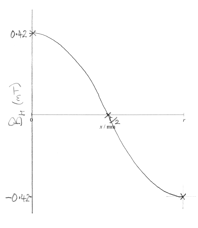
Finally we have Q3.7, which introduces another variation, Experiment 4, in which the two coils have the same current magnitude but now with Coil 2’s current reversed, meaning that the magnetic field of Coil 2 will be reversed with respect to Coil 1. You are provided with a bare x-axis and are asked to sketch a graph, with numerical values, showing the variation of magnetic flux density from x = 0 to x = r for this configuration.

The x-axis scale extends from the centre of Coil 1 (x = 0) to the centre of Coil 2 (x = r). Given that the currents in the two coils are of equal magnitude but in opposite directions, we would surely expect the peak magnetic flux densities to have the same values but with one being positive (Coil 1, at x = 0) and the other being negative (Coil 2, at x = r).

The peak value can be determined from Figure 11 by subtracting (because the fields are in opposite directions) the two magnetic flux densities. I read 0.655 mT as the value for Coil 1 (at x = 0) and 0.235 mT for Coil 2 (also at x = 0) giving a subtracted value of 0.42 mT. The same exercise can be repeated at x = r but I used symmetry to deduce the minimum value would have the same magnitude and therefore must be –0.42 mT.

The question then is; what happens in between? Logically we would expect zero magnetic flux density at the mid-point (x = r/2) and the shape of the curve should be sinusoidal, not a straight line. This can be deduced by recognising that the values at x = 0 and x = r are turning points so the connecting line must be a curve.

To score full marks you needed to label the y-axis correctly and mark the maximum and minimum values (0.42 mT and –0.42 mT respectively) with the x-axis intercept at r/2 and a smooth curved line through these points, as shown below.

I should add that the mark scheme expected the peak values to be 0.43 mT with a tolerance of +/-0.01 mT, which makes my value of 0.42 mT acceptable but not perfect. More importantly, a straight line could still score two marks provided that you labelled the y-axis correctly and had the right intercept on the x-axis. Well done if you got all three marks.

A full copy of the mark scheme for this paper can be downloaded here.