Determination of ‘little-g’

One of my favourite experiments in GCSE physics is a practical that seems to have fallen from favour in recent years – but it’s still worth exploring. The experiment involves using a ticker-timer to make dots at regular time intervals (0.02 s apart) on a strip of tape that is attached to a moving object. By measuring the distance between the dots it is simple to calculate the object’s speed (or velocity, since the tape has a fixed direction) at any given moment in time.

Using the fact that 0.02 is the same as 1/50, the usual equation (speed = distance / time) can be rewritten as; speed = 50 x distance. So if the distance between two dots is 20 mm, we know the average speed in that 0.02 s interval was 1000 mm/s (1 m/s).

If we then compare adjacent values for speed, we can determine the object’s acceleration, which is defined as the change in speed divided by the time taken. The time interval between successive periods of 0.02 s is, of course, 0.02 s so the acceleration equation becomes; acceleration = 50 x (change in speed).

Let’s look at an example… If an object moves 20 mm in the first 0.02 s then moves 25 mm in the second 0.02 s, we can calculate its two speeds to be 1 m/s (as above) and 1.25 m/s (using the same method). The object’s acceleration is therefore given by the calculation 50 x (1.25 – 1.00), which is 12.5 m/s².

This should all be fairly obvious but it is only the start of what is possible with ticker-tape analysis. In particular, we are able to track changes in the object’s motion in detail by looking at the distances between the marked dots over a longer period of time. This is commonly done as a way to determine the acceleration due to gravity, known as ‘little-g’ (* see footnote).

All of which brings us to a little project that interested readers may like to attempt. If you are on a half-term break, then I hope this will be a nice task to lubricate your mental cogs!

I’ve dropped a mass, with ticker tape attached, and cut the trace into lengths that have been stuck on graph paper for ease of measuring. In the diagram below, the original sections are shown on the left and my measurements for some of the individual distances are shown on the right. You will notice that there is a steady increase in the distance between the dots at first but at the end of the drop there appears to be some random variation.

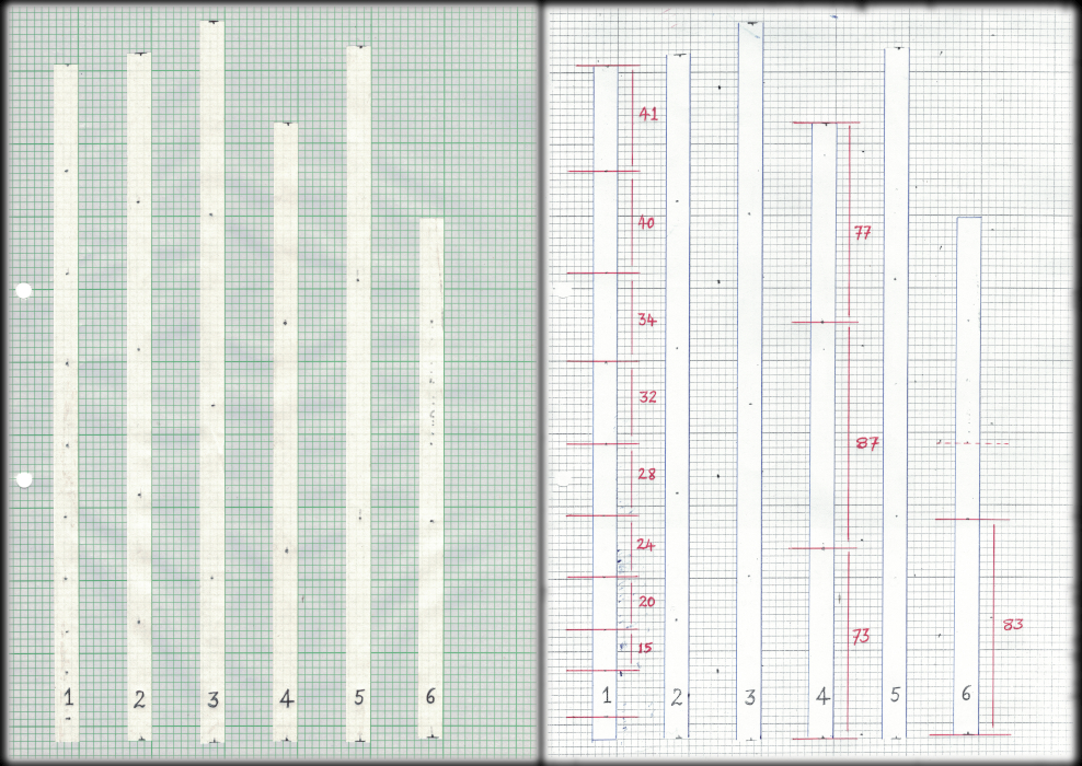
You can click on the illustration to download a high-resolution PDF with the original sections. You can then use this document to make your own measurements for the distances between successive dots. Your distances should (roughly) match my marked examples, +/- 1 mm, on the right-hand side of the illustration above. I’ve deliberately not given all the lengths I measured as it is important for you to make some measurements of your own! But if you don’t want to do any measurements, the first column of distances I’ve marked will provide enough data for you to do the analysis that follows.

The next step is to plot a graph with time (in intervals of 0.02 s) on the x-axis and mean speed, converted to metres-per-second, on the y-axis.

The full tape will give you 24 time markers (going from 0.02 s to 0.48 s) and speed values that reach a maximum of about 4.5 m/s. If you want to download some graph paper for this exercise then click here. Alternatively, you may decide to use spreadsheet analysis software, such as Microsoft Excel or LibreOffice Calc.

The acceleration of the falling mass is given by the gradient of the (linear) line-of-best-fit. The textbook value is 9.8 m/s² (often rounded to 10 m/s²) but your value should be less than this and will probably be in the range 8 – 9 m/s².

Ticker-tape analysis can also be used to investigate the motion of a dynamics trolley rolling down a ramp at different angles of tilt, or with different accelerating weights attached by a string that runs over a desk pulley. It can even be used to investigate whether all masses fall with the same acceleration by dropping, say, hooped masses of 100 g, 200 g, 500 g and 1 kg.

We all know, I hope, that objects should accelerate at the same rate regardless of their mass but that may not be true in practice – here on Earth, at least. That qualification should help you to explain the discrepancy between the textbook and experimental values, highlighted above. If you need a further hint, watch this video from the Apollo 15 moon mission. (By the way, if the moon landings were faked, as some people claim, then how did NASA manage to capture this footage?)

* Footnote: Whereas ‘little-g’ is the term used for the gravitational acceleration arising from the mass of a specific planet or other astronomical body, ‘big-G’ is the universal gravitational constant that has the same value everywhere. Or maybe not… The exact value of G may have changed over time and there is some uncertainty regarding its current value when measured by different experiments, as you can read here.