Acceleration and Distance

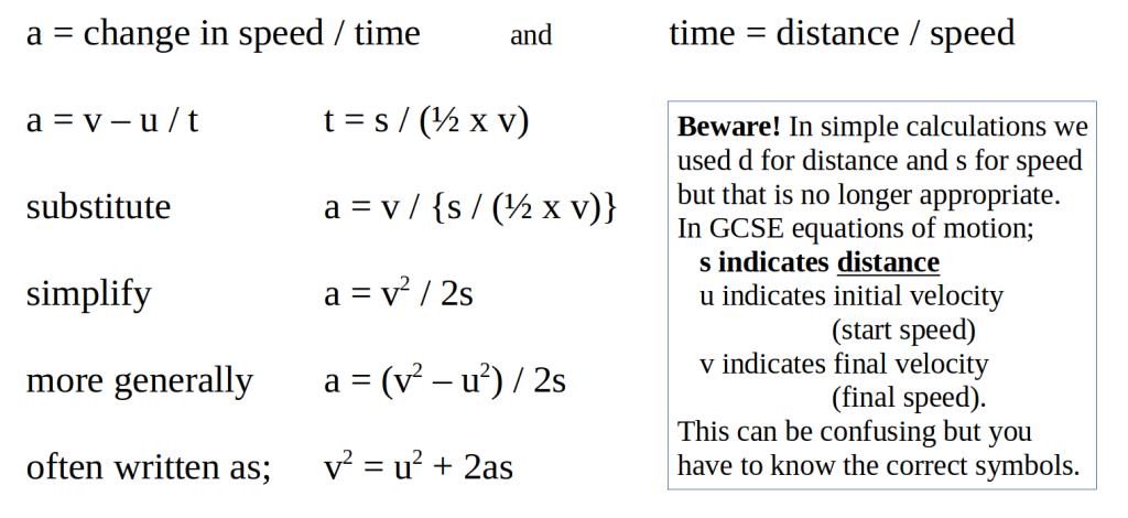
To find acceleration without measuring time, we can use a combination of the object’s mean speed and distance-moved as a substitute for time. We already know that speed is calculated as distance divided by time, so we can rearrange this equation to calculate time as distance divided by speed. Of course, the speed of an accelerating object is changing but we can still carry out the calculation if we know the object’s mean speed.

There is a very useful trick we can employ here: if an object starts from stationary and has constant acceleration, its mean speed will be equal to half of the speed that we measure at a certain distance. Why? Because to calculate the mean speed we add the start speed to the final speed then divide by two. The start speed is zero, so the mean speed is half of the final speed.

We can combine these facts to produce an equation that links acceleration to velocity (speed) and distance, as shown below. Note: you can skip this bit if it looks scary!

You do not have to remember this method or even the final equation: you just need to be able to select and use the equation at the appropriate time.

To apply this method, we can use light-gates to measure the speed of a model race car at different distances from the start of a straight-line sprint. If we are given speed values that were recorded at known distances then we can just substitute into the provided equation and solve to calculate the acceleration.

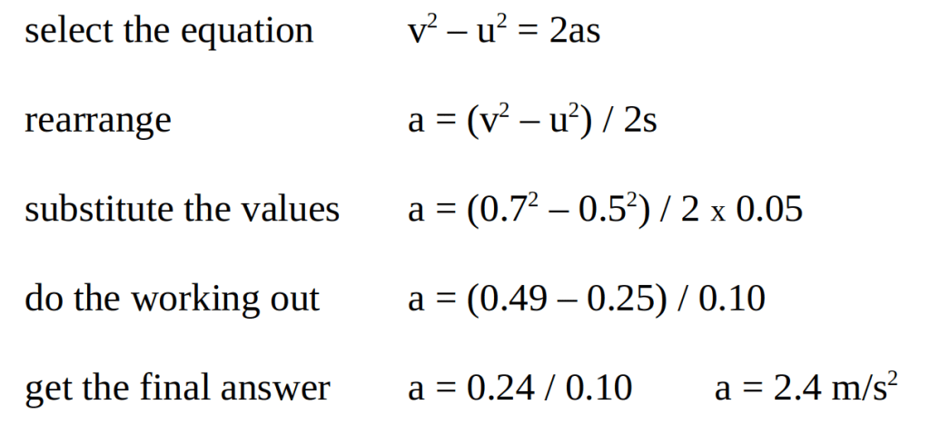
For example, suppose that a model race car has speeds of 0.5 m/s and 0.7 m/s at two positions that were 10 cm and 15 cm from the start. What is the acceleration of the car?

Before doing any calculations, find the distance between the two measurements (5 cm) and convert that distance to metres (0.05 m) then proceed as follows;

You could also be asked to analyse a graph to find the acceleration based on speed-distance data. Note that the graph must have speed-squared on the y-axis, not simply speed. This is illustrated in the two graphs below, where the speed graph (left) has a curved trend line but the same data plotted on a speed-squared graph (right) fits a linear trend line.

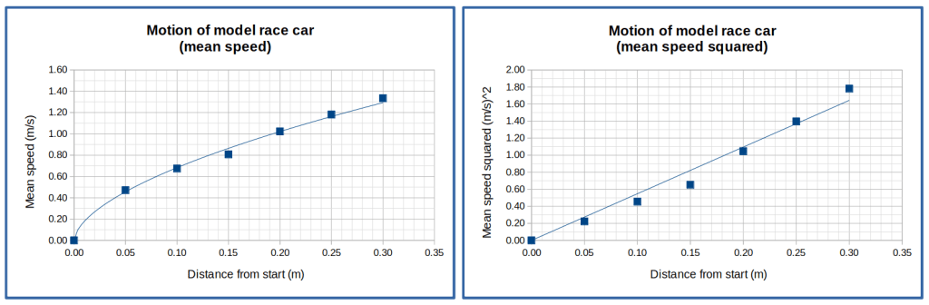
I’ll leave it to readers who are interested in the maths to explain why the gradient of the straight line is equal to double the object’s acceleration. This means that if you measure the gradient, then halve the value, you will get the object’s acceleration. Remember that the gradient must be measured using points that are on the line of best fit, not the original data.

The trend line goes through the point (0.09, 0.50) and the point (0.22, 1.20) so the gradient is given by (1.20 – 0.50) / (0.22 – 0.09). This expression simplifies to 0.70/ 0.13, which works out to 5.4. That value needs to be halved to get acceleration of the model car, which is therefore 2.7 m/s². This answer is slightly higher than the value calculated earlier but you will notice that the trend line is steeper above the two distance values used, which were 0.10 m and 0.15 m, so the discrepancy is not surprising. You should be able to explain why the value taken from the graph is likely to be more accurate (closer to the true value).

This completes our mini-series looking at motion. Next, we will look at the connection between unbalanced forces and changes in motion, which follows logically from this work.

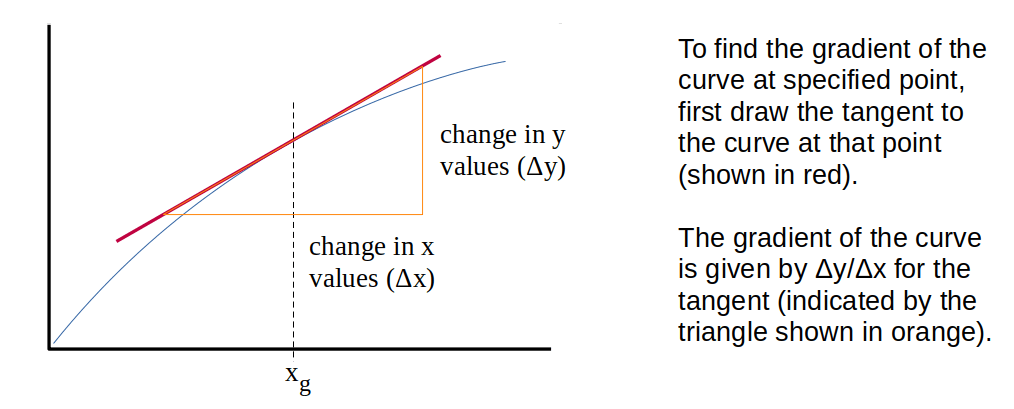
As a final comment, before moving on, it is important to add that gradients can be calculated for curved lines as well as straight lines. The method is the same – once an equivalent straight line has been identified. This is done by drawing a tangent to the curve at the point where the gradient is to be measured. The gradient of the tangent is equal to the gradient of the curve at that point, as illustrated in the diagram below.